Quickstart

Installation

pip install dpg

DPG requires Python 3.10+.

If you want graph rendering, install the system Graphviz package as well so the dot executable is available on your PATH.

For local development installs and longer setup notes, see docs/README.md.

Minimal example

The simplest way to use DPG is through DPGExplainer:

from sklearn.ensemble import RandomForestClassifier, GradientBoostingClassifier
from sklearn.datasets import load_iris
from dpg import DPGExplainer

# 1. Train any tree-based ensemble (RandomForest, GradientBoosting, AdaBoost, etc.)
X, y = load_iris(return_X_y=True, as_frame=True)
# model = RandomForestClassifier(n_estimators=5, random_state=42).fit(X, y)
model = GradientBoostingClassifier(n_estimators=5, random_state=42).fit(X, y)

# 2. Create the explainer (automatic model adaptation happens here)
explainer = DPGExplainer(
    model,
    feature_names=X.columns.tolist(),
    target_names=["setosa", "versicolor", "virginica"],
)

# 3. Fit (extract the graph from training paths)
explainer.fit(X.values)
explanation = explainer.explain_global()

# 4. Inspect metrics
print(explanation.node_metrics.head())
print(explanation.edge_metrics.head())

# 5. Visualise
explainer.plot(explanation, save_dir="results/")

What DPGExplainer returns

explainer.explain_global() returns a dpg.DPGExplanation dataclass with:

Attribute	Type	Description
graph	nx.DiGraph	NetworkX directed graph
dot	graphviz.Digraph	Graphviz rendering object
node_metrics	pd.DataFrame	Per-node betweenness, LRC, degree, …
edge_metrics	pd.DataFrame	Per-edge weight, source/target labels
class_boundaries	dict	Per-class feature constraint ranges
communities	dict	Optional community assignments

Configuration

DPG can be configured via a YAML file or a dict:

explainer = DPGExplainer(
    model,
    feature_names=X.columns.tolist(),
    dpg_config={
        "dpg": {
            "default": {
                "perc_var": 0.001,      # minimum path frequency (0-1)
                "decimal_threshold": 2, # rounding for thresholds
                "n_jobs": -1,           # -1 = all CPU cores
            }
        }
    },
)

You can also configure how the graph is constructed:

explainer = DPGExplainer(
    model,
    feature_names=X.columns.tolist(),
    dpg_config={
        "dpg": {
            "default": {
                "perc_var": 1e-9,
                "decimal_threshold": 6,
                "n_jobs": -1,
            },
            "graph_construction": {
                "mode": "execution_trace",  # or "aggregated_transitions"
            },
        }
    },
)

• aggregated_transitions: default global DPG behavior.

• execution_trace: trace-first construction, useful for local path inspection.

Supported Models

DPGExplainer works with a wide range of scikit-learn tree-based ensemble models:

Classification:

• ✅ RandomForestClassifier

• ✅ GradientBoostingClassifier (NEW!)

• ✅ ExtraTreesClassifier

• ✅ AdaBoostClassifier

• ✅ BaggingClassifier

Regression:

• ✅ RandomForestRegressor

• ✅ GradientBoostingRegressor (NEW!)

• ✅ ExtraTreesRegressor

• ✅ AdaBoostRegressor

All models work automatically without any special configuration. DPGExplainer detects the model type and handles differences internally.

For a complete list of models and detailed configuration options, see Supported Models.

Local explanations

After fitting the explainer, you can inspect one sample at a time:

local = explainer.explain_local(sample=X.iloc[0].values, sample_id=0)

print(local.majority_vote)
print(local.class_votes)
print(local.sample_confidence)

local_df = explainer.local_path_dataframe(local)
print(local_df.head())

Path labels remain in DPG format such as Class 0, while local.class_votes and local.majority_vote use normalized class names such as 0.

To render the local paths on top of the fitted DPG:

explainer.plot_local_on_dpg(
    "iris_local_sample0",
    local_explanation=local,
    true_class_label=str(y.iloc[0]),
    save_dir="results/",
    theme="dpg",
    palette="olive",
    show=False,
)

See examples/local_explanation_iris.py for a minimal runnable script.

Faithfulness evaluation

DPG can evaluate local explanations against the fitted black-box model:

details = explainer.evaluate_faithfulness(
    X_test,
    y_true=y_test,
    return_details=True,
)

print(details["faithfulness_score"])
print(details["output_fidelity"])
print(details["mean_trace_coverage_score"])
print(details["mean_recombination_rate"])

This API reports:

• output_fidelity: agreement between the local explanation and the model

• structural metrics such as trace coverage and recombination

• semantic metrics such as evidence margin

• a composite faithfulness_score

Notes:

• the composite score is a heuristic summary, not a calibrated probability

• output_fidelity measures agreement with the black-box model

• local_accuracy is only available when y_true is supplied

• structural faithfulness here is about recovering executed decision traces

Visualisation options

For a complete gallery of available graph and chart outputs, see Visualization.

The example outputs below use the themed DPG palette.

from dpg import plot_dpg, plot_lrc_vs_rf_importance, plot_top_lrc_predicate_splits

# Basic DPG plot
plot_dpg(
    "iris_dpg",
    explanation.dot,
    explanation.node_metrics,
    explanation.edge_metrics,
    save_dir="results/",
    attribute="Local reaching centrality",  # color by LRC
    theme="dpg",
    palette="olive",
    layout_template="vertical",
    label_mode="wrapped",
    readability="presentation",
    fig_size=(14, 14),
    title="Iris Decision Predicate Graph by Local Reaching Centrality",
)

# Compare DPG importance vs Random Forest importance
plot_lrc_vs_rf_importance(
    explanation,
    model,
    X,
    dataset_name="Iris",
    theme="dpg",
    palette="olive",
)

# Visualise top predicate split lines in feature space
plot_top_lrc_predicate_splits(
    explanation,
    X,
    y,
    dataset_name="Iris",
    theme="dpg",
    palette="olive",
)

The theming API also supports theme="legacy" and palette="default" if you want a more neutral look.

Example outputs:

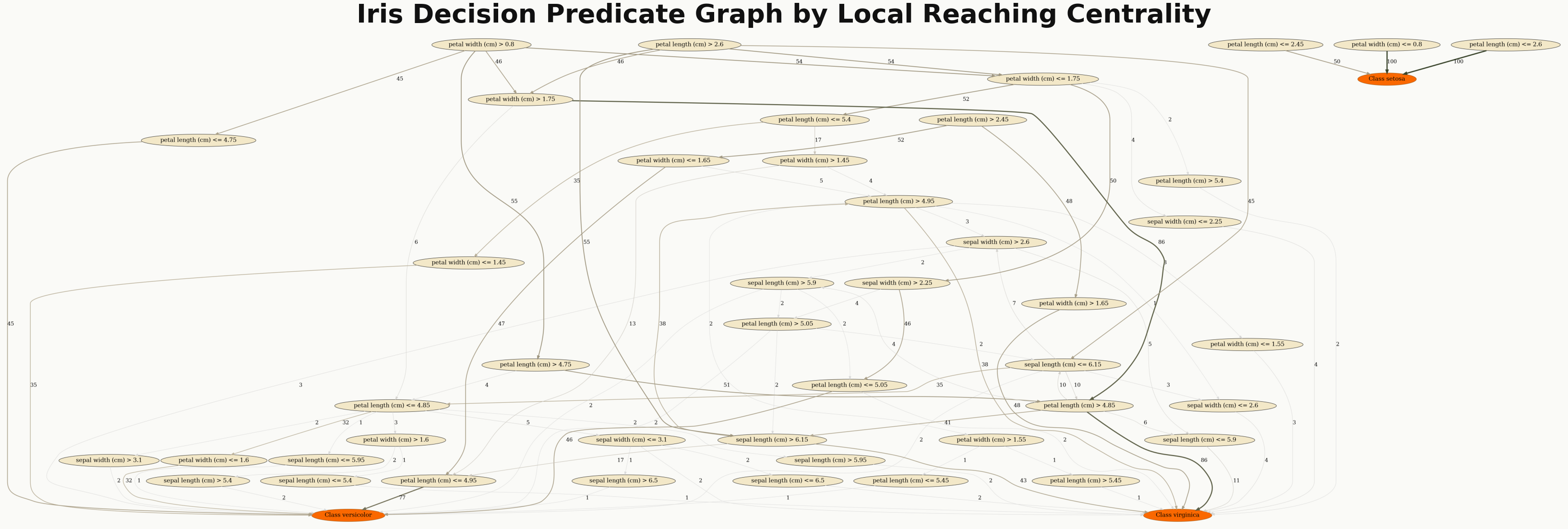
Decision Predicate Graph colored by Local Reaching Centrality.

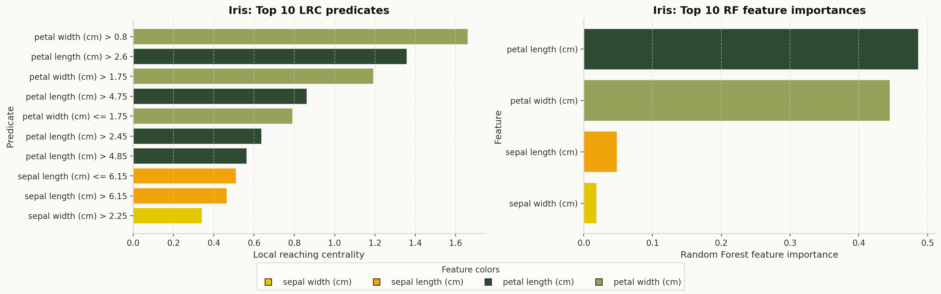
DPG-based feature importance compared with Random Forest feature importance.

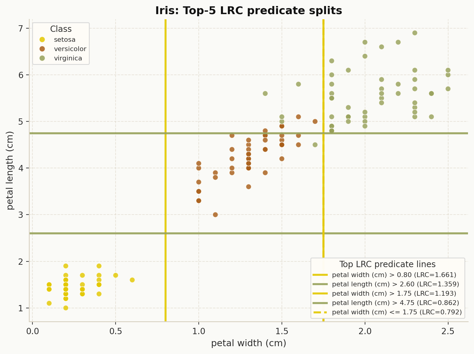
Top predicate split lines in feature space ranked by Local Reaching Centrality.

scikit-learn compatible pipeline

DPG also ships a scikit-learn Transformer wrapper:

from dpg.sklearn_dpg import DPGTransformer
from sklearn.pipeline import Pipeline

pipe = Pipeline([
    ("dpg", DPGTransformer(model, feature_names=X.columns.tolist())),
])